Sign up for our newsletter to receive these emails in your inbox.

---

Summary: The Simon–Ehrlich wager famously demonstrated that population growth does not lead to resource scarcity but instead drives innovation and abundance. Since 1900, the production of five metals featured in the bet has risen dramatically. This bolsters Julian Simon’s argument that human ingenuity and technological progress enable us to produce more resources at lower costs, ensuring greater abundance even as populations grow.

---

Hannah Richie at OurWorldinData.org recently published an insightful article on the five metals featured in the Simon–Ehrlich wager. In 1990, Paul Ehrlich lost the 10-year bet and had to write a check to Julian Simon for $576.07. Simon had let Ehrlich pick the five metals in 1980 when the bet started. The payment reflected the inflation-adjusted decline of 36 percent in the average price of the five metals over the decade. This was despite an extraordinary global population increase during the 1980s of 850 million people (19 percent)—the largest growth in human history. Yet, even with this surge, resource prices dropped, reinforcing Simon’s argument that human population growth, coupled with ingenuity and the freedom to innovate, drives resource abundance rather than scarcity.

Richie highlights an important trend: The long-term abundance of these metals has increased significantly. Take a look at the staggering growth in their production since the early 1900s:

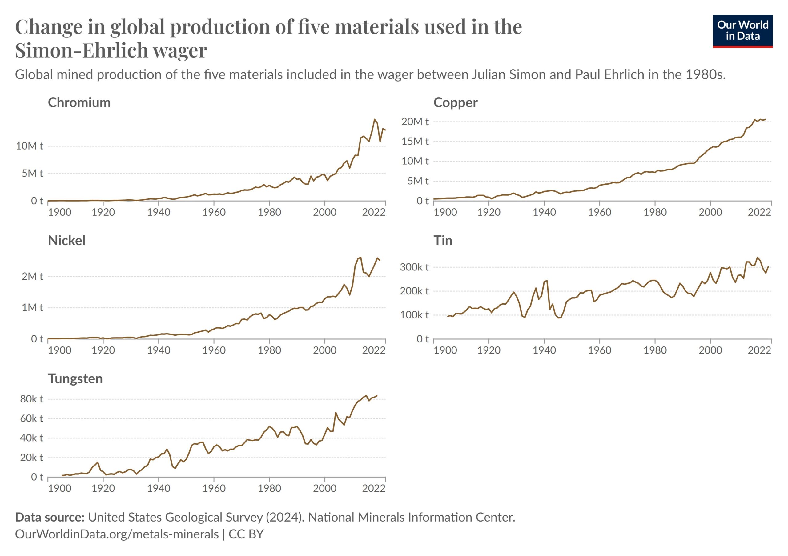
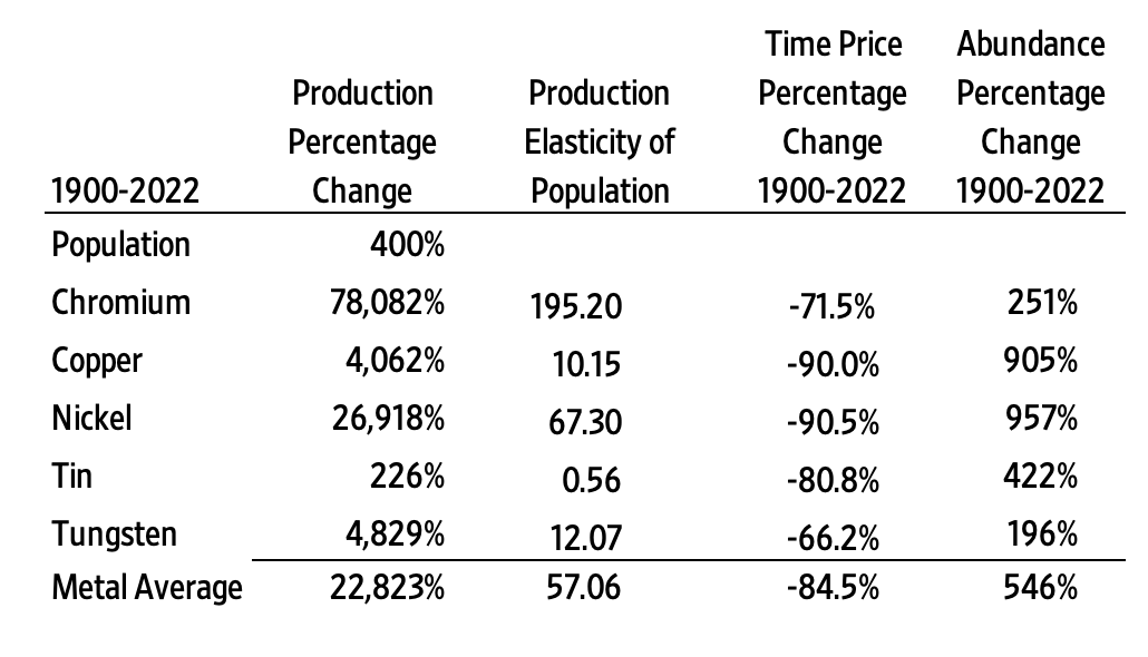
Between 1900 and 2000, the global population grew by 400 percent, from 1.6 billion to 8 billion. During the same period, the production of the five metals soared: Chromium increased by an astounding 78,082 percent, copper by 4,062 percent, nickel by 26,918 percent, tin by 226 percent, and tungsten by 4,829 percent. On average, production of these metals rose by 22,823 percent.

The relationship between population growth and resource production is captured by the production elasticity of the population. It is the ratio of the percentage change in production divided by the percentage change in population. On average, every 1 percent increase in population corresponded to a 57.06 percent increase in the production of these five metals.

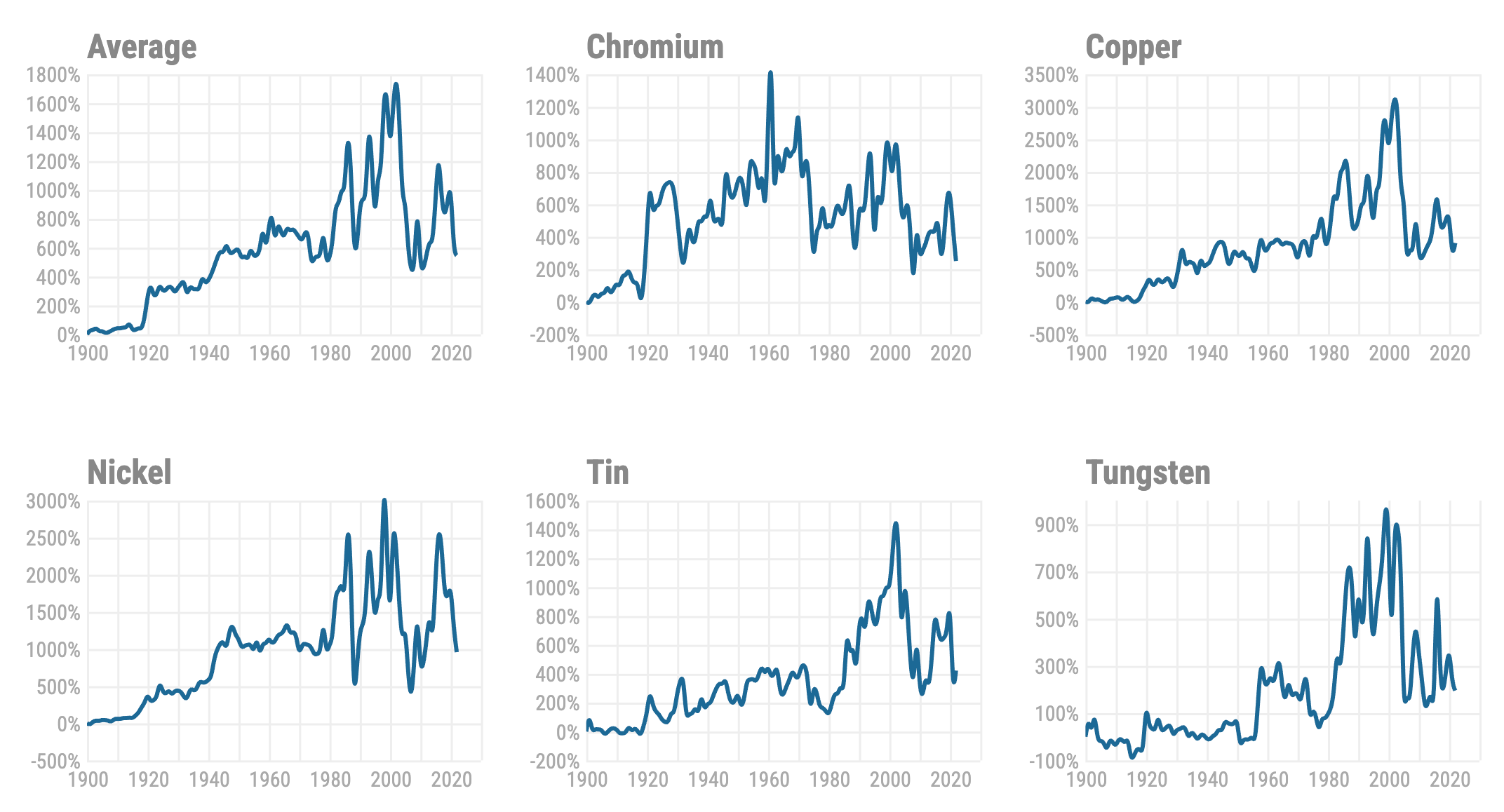
In our book Superabundance, we compared the time prices of these five metals for blue-collar workers from 1900 to 2018 and have since updated the data to 2022.

The charts below detail the growth in abundance for each resource since 1900. Please note that vertical scales differ across the charts. The charts generally show the effects of 9/11, the financial crisis of 2008, and COVID-19 lockdown policies.

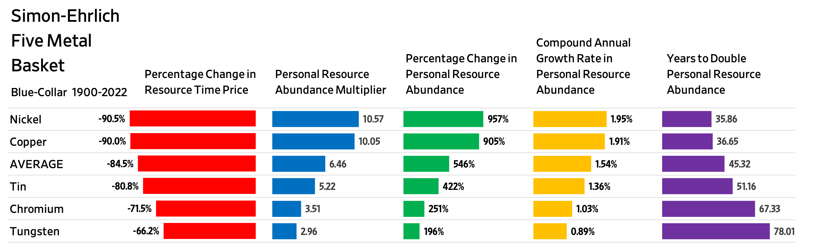
This table summarizes our findings.

From 1900 to 2022, the global population increased by 400 percent. Over the same period, the abundance of these five metals increased by an average of 546 percent, demonstrating that abundance has grown 36.5 percent faster than the population.

Some have suggested that Simon was just lucky. This is why looking at a much longer time period reveals underlying trends behind temporary fluctuations.

These data reinforce Simon’s prediction: The more people, the more we produce, and the lower the prices.

Tip of the hat: Max More

This article was published at Gale Winds on 1/14/2025.

The Simon Abundance Index (SAI) quantifies and measures the relationship between resources and population. The SAI converts the relative abundance of 50 basic commodities and the global population into a single value. The index started in 1980 with a base value of 100. In 2023, the SAI stood at 609.4, indicating that resources have become 509.4 percent more abundant over the past 43 years. All 50 commodities were more abundant in 2023 than in 1980.

Figure 1: The Simon Abundance Index: 1980–2023 (1980 = 100)

The SAI is based on the ideas of University of Maryland economist and Cato Institute senior fellow Julian Simon, who pioneered research on and analysis of the relationship between population growth and resource abundance. If resources are finite, Simon’s opponents argued, then an increase in population should lead to higher prices and scarcity. Yet Simon discovered through exhaustive research over many years that the opposite was true. As the global population increased, virtually all resources became more abundant. How is that possible?

Simon recognized that raw materials without the knowledge of how to use them have no economic value. It is knowledge that transforms raw materials into resources, and new knowledge is potentially limitless. Simon also understood that it is only human beings who discover and create knowledge. Therefore, resources can grow infinitely and indefinitely. In fact, human beings are the ultimate resource.

Visualizing the Change

Resource abundance can be measured at both the personal level and the population level. We can use a pizza analogy to understand how that works. Personal-level abundance measures the size of an individual pizza slice. Population-level abundance measures the size of the entire pizza pie. The pizza pie can get larger in two ways: the slices can get larger, or the number of slices can increase. Both can happen at the same time.

Growth in resource abundance can be illustrated by comparing two box charts. Create the first chart, representing the population on the horizontal axis and personal resource abundance on the vertical axis. Draw a yellow square to represent the start year of 1980. Index both population and personal resource abundance to a value of one. Then draw a second chart for the end year of 2023. Use blue to distinguish this second chart. Scale it horizontally for the growth in population and vertically for the growth in personal resource abundance from 1980. Finally, overlay the yellow start-year chart on the blue end-year chart to see the difference in resource abundance between 1980 and 2023.

Figure 2: Visualization of the Relationship between Global Population Growth and Personal Resource Abundance of the 50 Basic Commodities (1980–2023)

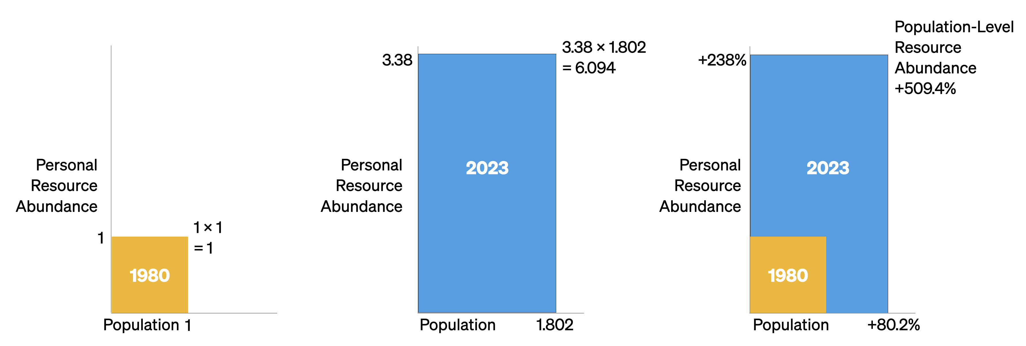
Between 1980 and 2023, the average time price of the 50 basic commodities fell by 70.4 percent. For the time required to earn the money to buy one unit of this commodity basket in 1980, you would get 3.38 units in 2023. Consequently, the height of the vertical personal resource abundance axis in the blue box has risen to 3.38. Moreover, during this 43-year period, the world’s population grew by 3.6 billion, from 4.4 billion to over 8 billion, indicating an 80.2 percent increase. As such, the width of the blue box on the horizontal axis has expanded to 1.802. The size of the blue box, therefore, has grown to 3.38 by 1.802, or 6.094 (see the middle box in Figure 2).

As the box on the right shows, personal resource abundance grew by 238 percent; the population grew by 80.2 percent. The yellow start box has a size of 1.0, while the blue end box has a size of 6.094. That represents a 509.4 percent increase in population-level resource abundance. Population-level resource abundance grew at a compound annual rate of 4.3 percent over this 43-year period. Also note that every 1-percentage-point increase in population corresponded to a 6.35-percentage-point increase in population-level resource abundance (509.4 ÷ 80.2 = 6.35).

Individual Commodity Changes: 1980–2023

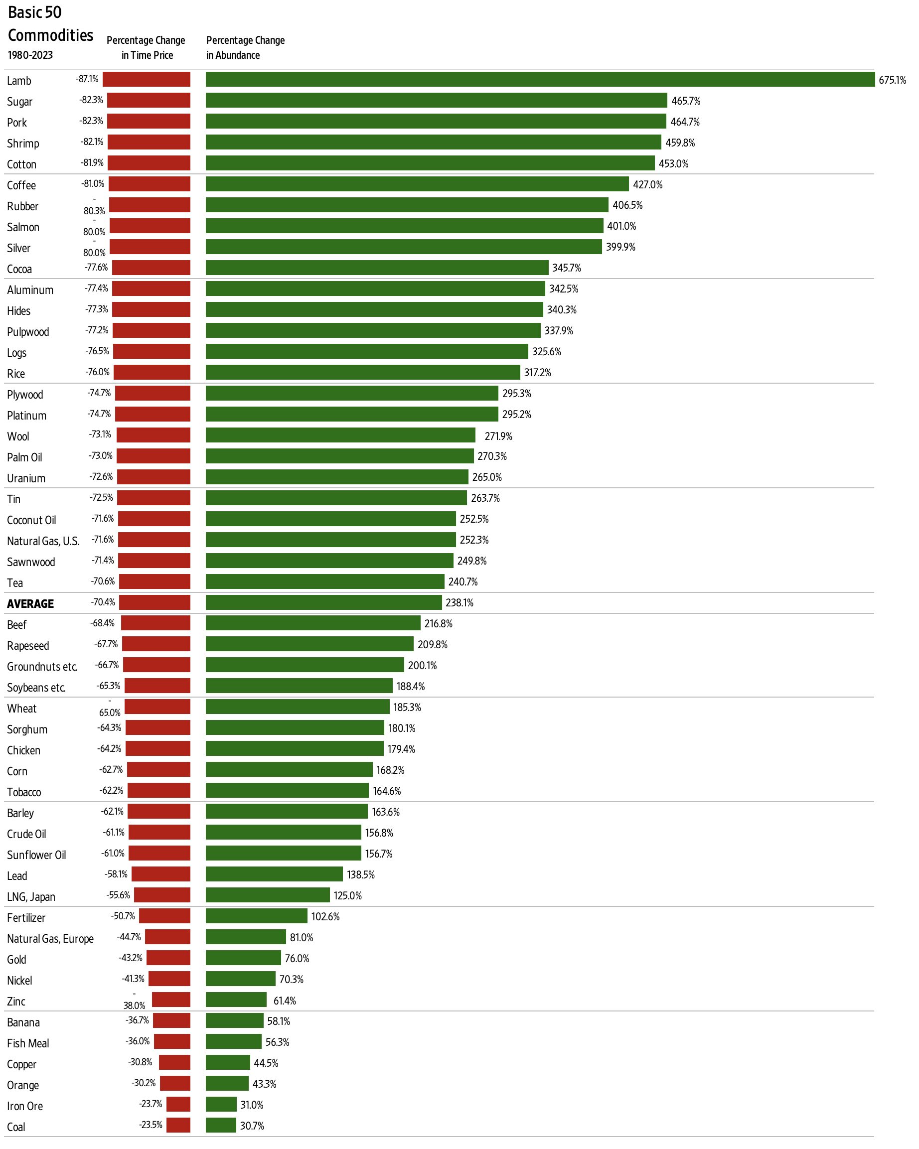
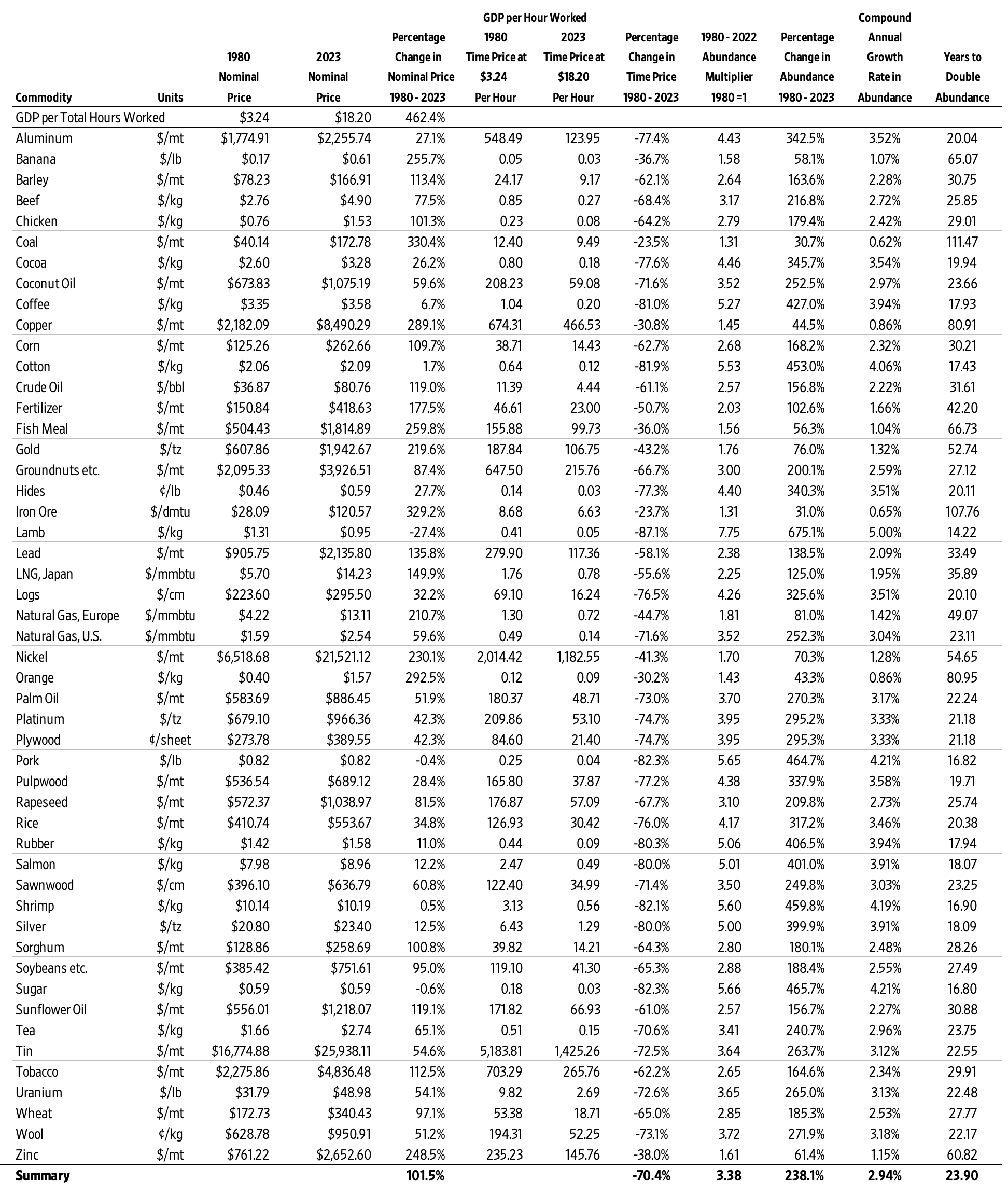
As noted, the average time price of the 50 basic commodities fell by 70.4 percent between 1980 and 2023. As such, the 50 commodities became 238.1 percent more abundant (on average). Lamb grew most abundant (675.1 percent), while the abundance of coal grew the least (30.7 percent).

Figure 3: Individual Commodities, Percentage Change in Time Price and Percentage Change in Abundance: 1980–2023

Individual Commodity Changes: 2022–2023

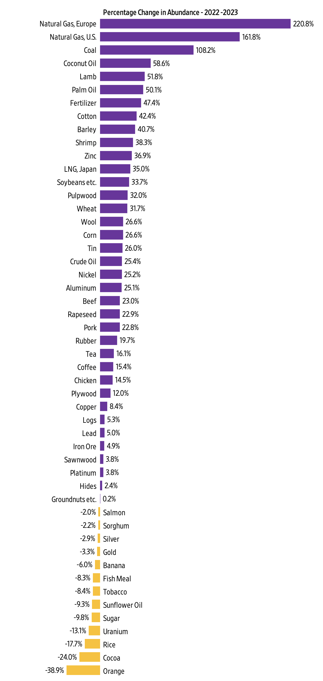
The SAI increased from a value of 520.1 in 2022 to 609.4 in 2023, indicating a 17.1 percent increase. Over those 12 months, 37 of the 50 commodities in the data set increased in abundance, while 13 decreased in abundance. Abundance ranged from a 220.8 percent increase for natural gas in Europe to a 38.9 percent decrease for oranges.

Figure 4: Individual Commodities, Percentage Change in Abundance: 2022–2023

Conclusion

After a sharp downturn between 2021 and 2022, which was caused by the COVID-19 pandemic, government lockdowns and accompanying monetary expansion, and the Russian invasion of Ukraine, the SAI is making a strong recovery. As noted, since 1980 resource abundance has been increasing at a much faster rate than population. We call that relationship superabundance. We explore this topic in our book Superabundance: The Story of Population Growth, Innovation, and Human Flourishing on an Infinitely Bountiful Planet.

Appendix A: Alternative Figure 1 with a Regression Line, Equation, R-Square, and Population

Appendix B: The Basic 50 Commodities Analysis: 1980–2023

Appendix C: Why Time Is Better Than Money for Measuring Resource Abundance

To better understand changes in our standard of living, we must move from thinking in quantities to thinking in prices. While the quantities of a resource are important, economists think in prices. This is because prices contain more information than quantities. Prices indicate if a product is becoming more or less abundant.

But prices can be distorted by inflation. Economists attempt to adjust for inflation by converting a current or nominal price into a real or constant price. This process can be subjective and contentious, however. To overcome such problems, we use time prices. What is most important to consider is how much time it takes to earn the money to buy a product. A time price is simply the nominal money price divided by the nominal hourly income. Money prices are expressed in dollars and cents, while time prices are expressed in hours and minutes. There are six reasons time is a better way than money to measure prices.

First, time prices contain more information than money prices do. Since innovation lowers prices and increases wages, time prices more fully capture the benefits of valuable new knowledge and the growth in human capital. To just look at prices without also looking at wages tells only half the story. Time prices make it easier to see the whole picture.

Second, time prices transcend the complications associated with converting nominal prices to real prices. Time prices avoid subjective and disputed adjustments such as the Consumer Price Index (CPI), the GDP Deflator or Implicit Price Deflator (IPD), the Personal Consumption Expenditures price index (PCE), and the Purchasing Power Parity (PPP). Time prices use the nominal price and the nominal hourly income at each point in time, so inflation adjustments are not necessary.

Third, time prices can be calculated on any product with any currency at any time and in any place. This means you can compare the time price of bread in France in 1850 to the time price of bread in New York in 2023. Analysts are also free to select from a variety of hourly income rates to use as the denominator when calculating time prices.

Fourth, time is an objective and universal constant. As the American economist George Gilder has noted, the International System of Units (SI) has established seven key metrics, of which six are bounded in one way or another by the passage of time. As the only irreversible element in the universe, with directionality imparted by thermodynamic entropy, time is the ultimate frame of reference for almost all measured values.

Fifth, time cannot be inflated or counterfeited. It is both fixed and continuous.

Sixth, we have perfect equality of time with exactly 24 hours in a day. As such, we should be comparing time inequality, not income inequality. When we measure differences in time inequality instead of income inequality, we get an even more positive view of the global standards of living.

These six reasons make using time prices superior to using money prices for measuring resource abundance. Time prices are elegant, intuitive, and simple. They are the true prices we pay for the things we buy.

The World Bank and the International Monetary Fund (IMF) track and report nominal prices on a wide variety of basic commodities. Analysts can use any hourly wage rate series as the denominator to calculate the time price. For the SAI, we created a proxy for global hourly income by using data from the World Bank and the Conference Board to calculate nominal GDP per hour worked.

With this data, we calculated the time prices for all 50 of the basic commodities for each year and then compared the change in time prices over time. If time prices are decreasing, personal resource abundance is increasing. For example, if a resource’s time price decreases by 50 percent, then for the same amount of time you get twice as much, or 100 percent more. The abundance of that resource has doubled. Or, to use the pizza analogy, an individual slice is twice as large. If the population increases by 25 percent over the same period, there will be 25 percent more slices. The pizza pie will thus be 150 percent larger [(2.0 x 1.25) – 1].

Reading the news can leave you depressed and misinformed. It’s partisan, shallow, and, above all, hopelessly negative. As Steven Pinker from Harvard University quipped, “The news is a nonrandom sample of the worst events happening on the planet on a given day.”

So, why does Human Progress feature so many news items? And why did I compile them in this giant list? Here are a few reasons:

• Negative headlines get more clicks. Promoting positive stories provides a necessary balance to the torrent of negativity.
• Statistics are vital to a proper understanding of the world, but many find anecdotes more compelling.
• Many people acknowledge humanity’s progress compared to the past but remain unreasonably pessimistic about the present—not to mention the future. Positive news can help improve their state of mind.
• We have agency to make the world better. It is appropriate to recognize and be grateful for those who do.

Below is a nonrandom sample (n = ~1000) of positive news we collected this year, separated by topic area. Please scroll, skim, and click. Or—to be even more enlightened—read this blog post and then look through our collection of long-term trends and datasets.

Agriculture

Aquaculture

• The Future of Fish Farming Is on Land
• A Better Way to Get Oysters? Try Growing Them on Land
• How This Virginia Aquaculture Farm Raises Four Million Oysters for Market

Farming robots and drones

• The Farming Robots That Will Feed the World
• Lasers, Drones and AI: The Future of Weeding
• Flying Tractors Are a Window into Farming’s Future
• Meet the New Crop-Dusting Drones
• New Farming Robot Uses AI to Kill 100,000 Weeds per Hour
• Grain-Flinging Robot Goes into Granaries So Farmers Don’t Have To
• Robot Gardener Grows Plants as Well as Humans Do but Uses Less Water
• More Autonomous Robots to Hit Farms with Manufacturer’s US Expansion
• Use of AI-Based Robots on the Rise in Japanese Agriculture

Food abundance

• Downward Slide in Global Food Prices Continues
• Global Food Costs Mark One Year of Drops, at Odds with Inflation
• US Corn Farmers Defy a Scorching Summer to Grow Record Crop
• The Great Wheat Price Surge That Sputtered

Genetic modification

• Crispr Wants to Feed the World
• How CRISPR Could Help Save Crops from Devastation Caused by Pests
• Commercial Development of Gene-Edited Food Now Legal in England
• EU Weighs Easing GMO Rules in Climate and Food Security Push
• The European Union Is Finally Coming Around to Gene-Edited Seeds
• Crispr Sausage Gets FDA Green Light for Consumption
• Scientists Are Gene-Editing Flies to Fight Crop Damage
• Bird Flu: Scientists See Gene Editing Hope for Immune Chickens
• The First Crispr-Edited Salad Is Here
• New Kind of Chicken Lays Eggs That Don’t Have Allergy Protein
• Scientists Unlock Key to Drought-Resistant Wheat Plants with Longer Roots
• Scientists Breed Flame-Resistant Cotton
• Genetically Modified Bananas Out to Stop Cavendish Catastrophe
• Philippines Scientists Develop Climate-Resistant Rice
• Genome Editing Used to Create Disease-Resistant Rice
• Gene-Edited Yeast Is Taking Over Craft Beer
• Insulin Grown in Lettuce Can Be Taken Orally
• Shrinking Corn Could Help Farmers—and the Environment
• Philippines Approves Bt Cotton for Commercial Propagation
• CRISPR Crops Are Here
• The Turbo-Charged Plants That Could Boost Farm Output
• Mutant Tomato Could Save Crops around the World
• Can Science Finally Create a Decent Cup of Decaf?
• Building a Better Forest Tree with CRISPR Gene Editing

Indoor farming

• Indoor Farming Isn’t Just for the Rich
• Amazon Collaborates with Hippo Harvest on New Sustainable Greens Line
• NASA Research Is Unleashing a Vertical Farming Boom
• It’s Winter in Antarctica, but Scientists Just Grew Watermelons There
• Saudi City of Future Enlists Dutch Help to Grow Crops in Desert

Lab-grown produce

• Eating Chicken without Killing Chicken?
• Fish Filet Created via 3D Printer May Be Hitting Market in the Near Future
• Lab-Grown Bacon Startup Uncommon Raises $30 Million
• Lab-Grown Meat Gets a Key Ingredient: 3D Fat
• FDA Says Lab-Grown Chicken Is Safe to Eat
• Eternal Creates Chicken Breast Analogue Made with Nutritious and Cost-Effective Fungi
• Meatball from Long-Extinct Mammoth Created by Food Firm
• Lab-Grown Meat Is Finally Approved in the US. Here’s How You Can Get Some.
• Coming to a Store near You – Shoes Made of Lab-Grown Leather
• This Is What Food Made from Air, Water and Electricity Looks Like
• CRISPR Tech Could Bring Cheaper Beef to Your July 4 Cookout
• Petri-Dish Leather and Silk Spun from Sugar: Could Future Fashion Be Grown in a Lab?
• Lab-Grown Meat Startup Raises Funds for Speedy Pork Sausages
• Lab-Grown Meat Companies Want a World of Steak without Slaughter

Pollination

• A Biotech Startup Is Boosting Bee Endurance with Supplements
• U.S.D.A. Approves First Vaccine for Honeybees

Other innovations

• Fine Young Cannibals: Locust Study Could Lead to Better Pest Control
• Plant Virus Recruited to Save Crops from Root-Eating Nematodes
• Fern Proteins Fight Crop Pests, Could Usher In Potent New Insecticides
• Pig Cooling Pads and Weather Forecasts for Cows Are High-Tech Ways to Make Meat in a Warming World
• “This Could Be the Holy Grail to Replace Palm Oil” – Research Team
• Reduce Synthetic Fertilizers and Improve Yields? The Microbiome Revolution Comes to Agriculture
• Apple Revival: How Science Is Bringing Historic Varieties Back to Life

Conservation and Biodiversity

Big cats

• Cougars Are Heading East
• Elusive and Rare Leopard — Considered Extinct for 45 Years — Caught On Film in Turkey
• India Now Has 3,167 Tigers
• Signs of Recovery for the Critically-Endangered West African Lion
• “Extinct” Lion Spotted in Chad National Park
• Tiger Populations Grow in India and Bhutan
• Bhutan Announces 39.5% Increase in Snow Leopard Numbers
• Return of the Lions: Large Protected Areas in Africa Attract Apex Predator

Birds

• Mumbai Embraces Its Booming Flamingo Population
• Bird Flu Vaccine Authorized for Emergency Use in California Condors
• New Research Reveals Scale and Success of Seabird Recovery Efforts Worldwide
• Lehua Island Now Free of Invasive Rats
• ‘Constant Bird Song’ Result of Conservation on Mercury Islands
• After a Big Recovery, the Wood Stork May Soon Fly off the Endangered Species List
• Peregrine Falcons, Once Extremely Endangered, Now Stable in Iowa Skies
• One of Europe’s Most Endangered Birds Is Bouncing Back
• Lundy Island Wild Bird Numbers Soar
• Golden Eagles in Scotland at Highest Levels in 300 Years
• Maine’s Puffin Colonies Are Recovering
• Prehistoric Bird Once Thought Extinct Returns to New Zealand Wild
• ‘New Hope’: Tiny Galápagos Island Birds Make Promising Comeback
• Wild Swan Conservation Success Gives Cause for Hope
• First White-Tailed Eagle in 240 Years Born in England

Turtles

• Love of Sea Turtles Turns Philippine Poachers into Protectors
• Royal Turtles on Verge of Comeback in Cambodia
• Number of Sea Turtle Nests on Florida Coasts Exploding, Even Tripling in Some Regions
• Record-Breaking Number of Green Sea Turtle Nests Found on Texas Beaches This Year
• Record Year for Olive Ridley Turtles in Bangladesh
• Record-Breaking Number of Sea Turtle Nests Found on Jupiter-Area Beaches

Whales

• The Islands That Went from Whale Hunting to Whale Watching
• North Atlantic Right Whale Population Has Steadied
• Australia’s Annual Humpback Whale Migration Shows Massive Recovery
• How the Humpback Whale Made a Massive Comeback in the Salish Sea
• Blue Whales Are Thriving in California Waters – the Story of Their Amazing Comeback
• Blue Whales: Ocean Giants Return to “Safe” Tropical Haven

Other comebacks

• California County Sees Highest Number of Monarch Butterflies in More than 20 Years
• Western Monarch Count Tallies Over 330,000 Butterflies
• Monarch Butterfly Is Not Endangered, Conservation Authority Decides
• Moth on Brink of Extinction Found Flying at Secret Scottish Site
• “Extinct” Butterfly Species Reappears in UK
• Conservation Efforts Celebrated as 26 Australian Species No Longer Need Threatened Listing
• Uganda Sees Resurgence of Rhinos, Elephants, Buffaloes
• Rhino, Elephant Numbers Rising in Uganda after Years of Poaching
• Critically Endangered Porpoise Shows Signs of Recovery
• Investigation: There Is No Sixth Mass Extinction Going On
• Renowned Conservation Effort Restores Maine’s Puffin Colonies
• Black Rhino Populations Are Starting to Thrive in Zimbabwe for the First Time in Decades
• Tiny Bats Provide “Glimmer of Hope” against a Fungus That Threatened Entire Species
• Golden Paintbrush Delisted from Endangered Species Act Due to Recovery
• Alaska’s Sea Otters Have Made a Major Comeback
• First-Ever Images Prove “Lost Echidna” Not Extinct
• Rhino Numbers Rebound as Global Figures Reveal a Win for Conservation
• Giant Tortoises Are Once Again Flourishing at Isabela’s Alcedo Volcano
• Seals Are Making a Comeback in Belgium
• Unprecedented Conservation Triumph: Saiga Antelope Return from the Red List
• Rare Animal Thought to Be Extinct Suddenly Found by Dog on Beach
• Southern Africa Elephant Population Increases
• Australian Earless Dragon Last Seen in 1969 Rediscovered in Secret Location
• Meet the Kipunji: A Rare Primate Success Story in Tanzania
• Returning Giant Tortoises Are Helping Recreate the Galapagos Islands Darwin Saw
• Rare, Critically Endangered Gecko Making Dramatic Recovery in Caribbean
• Sharks Are Flourishing off of U.S. East Coast
• More Wild Atlantic Salmon Found in U.S. Rivers than Any Time in the Past Decade, Officials Say

Forests

• Palm Oil-Driven Deforestation Is Falling
• Colombia Deforestation Plummets as Peace Efforts Focus on Rainforest
• Significant Growth in China’s Mangrove Forests
• Indonesia, Malaysia Have Cut Deforestation in Half in Last Half-Decade
• Despite Severe Drought, Amazon Deforestation Continues to Slow
• New Tree Tech: Cutting-Edge Drones Give Reforestation a Helping Hand

Reefs

• “Unprecedented” Coral Disease Relief
• Scientists Discover Pristine Deep-Sea Galápagos Reef “Teeming with Life”
• Florida’s Coral Reef Supports Fishing, Tourism and Beaches. Can Science Save It?
• “Every Square Inch Is Covered in Life”: The Ageing Oil Rigs That Became Marine Oases
• Oysters Back from the Brink in Brisbane Thanks to Novel Restoration
• Australian Startup Using AI to Help Coral
• Pacific Coral Reef Shows Unprecedented Increase in Climate Resistance
• Google Wants You to Save Coral Reefs (with AI’s Help)

Rivers and lakes

• Dolphins Spotted Swimming in New York City’s Bronx River
• Wirral Fishermen in Dreamland as River Mersey Makes a Comeback
• Toronto’s Don River, Once Declared Dead, Is Roaring Back to Life
• Invertebrate Biodiversity Is Improving in England’s Rivers, Long-Term Trends Show
• The Great Salt Lake Seemed Like It Was Dying. But There’s Been a ‘Miraculous’ Shift

Surveillance and discovery

• Underwater Creatures: 5,000 New Species Found in the Pacific Ocean
• Ocean Census Aims to Discover 100,000 Previously Unknown Marine Species
• Forecast Warns When Sea Life Will Get Tangled in Nets — One Year in Advance
• A Map of Every Tree in Africa Will Help Monitor Deforestation
• Scientists Discover 380 New Species in Southeast Asia
• Vulture Surveillance System Alerts Zambian Park to Poisonings
• DNA Sucked into Air Filters Can Reveal What Plants and Animals Are Nearby
• Sound Recordings and AI Tell Us If Forests Are Recovering, New Study from Ecuador Shows
• ‘Only AI Made It Possible’: Scientists Hail Breakthrough in Tracking British Wildlife
• Researchers Have Identified a New Pack of Endangered Gray Wolves in California
• Racing Sailors Pick Up Parasite eDNA in Warm Water Samples
• AI Used to Deter Deer from Railway Tracks over Festive Period

Rewilding and conservation

• Beavers to Be Reintroduced in Hampshire for First Time in 400 Years
• Conservationists Are Saving America’s Prairies by Selling Them Off
• Race to Vaccinate Rare Wild Monkeys Gives Hope for Survival
• Mexican Wolf Program Is Making Strides after 25 Years of Effort
• Beavers to Return to London as Part of Urban Rewilding
• Koalas Are Dying from Chlamydia. A New Vaccine Effort Is Trying to Save Them
• A Pioneering Project Is Cleaning Up Abandoned Crab Traps
• Platypuses Return to Sydney’s Royal National Park after Disappearing for Decades
• Native Giraffes Make a Return to Angola
• Northern White Rhinos Are Set for Extinction. Only a Technological Moonshot Can Save Them.
• Carnivorous Plants Return to Lancashire Peatland after 100 Years
• Rare Butterflies Thriving in England after Reintroduction Bid
• Beavers to Return to England’s Nene Wetlands after 400 Years
• 500 Baby Sharks to Be Released: An Exclusive Look at an Unprecedented Mission
• Baby Beaver Born in London for First Time in 400 Years
• Barrington Wildlife Sanctuary Celebrates Birth of 500th Tasmanian Devil
• The Alternative Ivory Sources That Could Help Save Elephants
• Kavango-Zambèze, an Area of Stability for Elephants
• Adorable Robot Lawn Mower Can Help Save the Bees
• AI Becomes an Unlikely Wildlife Warrior

De-extinction

• Dodo Next in Line for De-extinction by Scientists Reviving the Mammoth
• A New Cloned Horse Offers Hope for Endangered Species
• First RNA Extracted from Extinct Species May Help Thylacine Resurrection

Culture and tolerance

Gender equality

• Saudi Arabia Is Making Historic Strides in Women’s Rights
• Women in Sierra Leone Can Finally Own Land
• Six Ways the Lives of Girls Are Improving
• Child Marriage Has Declined Globally

General wellbeing

• Americans Largely Satisfied With Their Personal Life
• Loneliness in U.S. Subsides From Pandemic High
• U.S. Workers Are Happier Than They’ve Been in Decades
• The Great Decline in Adolescent Risk Behaviours
• Young Driver Fatality Rates Have Fallen Sharply in the US
• Morality Is Declining, Right? Scientists Say That Idea Is an Illusion

LGBT

• Kenya’s LGBTQ Community Wins Bittersweet Victory in Battle for Rights
• Japan Is Hostile for LGBTQ People, but Attitudes Are Shifting.
• The Cook Islands Have Decriminalized Homosexuality
• Growing Global Acceptance of Gay and Lesbian People
• Estonia Set to Become First Ex-Soviet State to Back Gay Marriage
• Sri Lanka Supreme Court Clears Path to Decriminalize Homosexuality
• Majority Worldwide for First Time Says Their Area Is Good Place for Gay People to Live: Gallup
• Thailand’s Cabinet Approves a Bill to Grant Same-Sex Couples Equal Rights
• More Gay Men Can Give Blood as ‘One of the Most Significant Changes in Blood Banking History’ Gets Underway

Treatment of animals

• New Techology Could Save Male Chicks
• One-Off Injection May Provide Lifetime Contraception for Female Cats
• Dogs Born Today Will Be Cured of Cancer Thanks to Human Advances
• Could a Drug Give Your Pet More Dog Years?
• Largest Ever Canine Rabies Vaccination Drive in Cambodia

Energy and natural Resources

Fission

• NRC Certifies First U.S. Small Modular Reactor Design
• GE Hitachi and 3 Partners Announce First Commercial Contract for Grid-Scale SMR in North America
• Several Universities to Experiment with Micro Nuclear Power
• Modular Nuclear Plants Could Reshape Coal Country
• US Firm Agrees to Sell 24 Mini Nuclear Reactors to UK Customers
• Europe’s Most Powerful Nuclear Reactor Kicks Off in Finland
• Fourth Generation Nuclear Reactors Take a Big Step Forward
• Americans’ Support for Nuclear Energy Highest in a Decade
• Oklo’s Next Two Nuclear Power Plants Planned for Southern Ohio
• Nuclear-Powered Cargo Ships Are Trying to Stage a Comeback
• OpenAI’s Sam Altman Is Taking a Nuclear-Energy Startup Public
• The First US Nuclear Reactor Built from Scratch in Decades Enters Commercial Operation in Georgia
• Poland’s Environment Agency Greenlights Country’s First Nuclear Power Plant
• Sweden Plans “Massive” Expansion of Nuclear Energy
• US, UK to Push Pledge to Triple Nuclear Power by 2050 at COP28

Fusion

• Startups Try to Turn Laser Fusion Success into Clean Power Plants
• Nuclear Fusion Will Not Be Regulated the Same Way as Nuclear Fission
• The Israeli Plan to Fit a Fusion Reactor into a Container
• Helion Energy Will Provide Microsoft with Fusion Power Starting in 2028
• US Scientists Repeat Fusion Power Breakthrough
• 3 Laser Fusion Research Hubs Picked by Energy Department
• US Nuclear-Fusion Lab Enters New Era: Achieving “Ignition” Over and Over

Fossil fuels

• BP’s $4.1 Billion Bet on Renewable Natural Gas Gets Underway
• The United States Is Producing More Oil than Any Country in History

Other energy

• A New Battery Approach Holds Promise for Storing Intermittent Renewable Energy at Scale
• This Geothermal Startup Showed Its Wells Can Be Used Like a Giant Underground Battery
• Mini Hydro Company Raises $18M to Generate Power in Canals
• A Massive Geothermal Apartment Complex Is Going Up in Brooklyn, the First of Its Kind
• Scientists Find Way to Make Energy from Air Using Nearly Any Material
• Scientists Beam Solar Power to Earth from Space for First Time Ever
• Virtual Power Plants Are Coming to Save the Grid
• Energy Startup Says It Has Achieved Geothermal Tech Breakthrough
• Bill Gates Is Backing a Secret Startup Drilling for Limitless Clean Energy
• A Vast Untapped Green Energy Source Is Hiding beneath Your Feet
• There’s a Vast Source of Clean Energy beneath Our Feet. And a Race to Tap It.
• Solar Panels Could Be About to Get Much Better at Capturing Sunlight
• Here Come the Iron Batteries
• Electrified Cement Could Turn Houses and Roads into Nearly Limitless Batteries
• Geothermal Energy Storage Is Cost Competitive with Lithium-Ion Batteries, Pumped Hydro: Pilot
• America’s First “Enhanced” Geothermal Plant Just Got Up and Running
• The First Cargo Ship Running on Green Methanol Is Setting Sail

Recycling and resource efficiency

• Tiny Data Centre Used to Heat Public Swimming Pool
• Iceland’s Quest to Use 100 Percent of Its Fish Waste
• Amazon Appears to Be Cutting Down on Plastics
• Tesla Switches to Motors without Rare Earth Elements
• What If Your Tesla Could Run on Sodium?
• Polyester May Be the Ultimate Recyclable Fiber
• The Incredible Shrinking Energy Use of a Light Bulb
• Battery Maker Develops Futuristic Cobalt-Free Cell for Electric Cars
• The Gold Jewellery Made from Old Phones
• Using Bacteria to Dye Fabric Cuts Fashion Waste
• How a Simple Tag Helped India Save Fuel Worth $8.4 Billion
• Can Tech Stop India Wasting So Much of Its Harvest?
• AI Is Great at Recycling
• The T-shirt Chewing Enzyme Ready to Tackle Plastic Waste
• Microbes Discovered That Can Digest Plastics at Low Temperatures

Resource abundance

• Sweden Discovers Biggest Rare Earths Deposit in EU
• Cobalt, a Crucial Battery Material, Is Suddenly Superabundant
• Falling Lithium Prices Are Making Electric Cars More Affordable
• Sheep Creek Deposit’s Rare Earth Samples Exceed Highest Grades in US
• EU Hails Discovery of Massive Phosphate Rock Deposit in Norway
• IEA Says Critical Minerals Supply Could Pull Close to Demand by 2030
• World’s Largest White Hydrogen Deposit Found in France
• Lithium Rout Deepens with Battery Metal Now Down 75% This Year
• Salton Sea Could Meet Nation’s Lithium Demand for Decades, Study Finds
• NASA Sensor Produces First Global Maps of Surface Minerals in Arid Regions
• AI Assists in Discovery of Lithium for Electric Vehicle Batteries
• Diamond Prices Are in Free Fall in One Key Corner of the Market
• The Floating Desalination Machines Powered by the Waves

Environment and pollution

Climate change

• Volcanic Microbe Eats CO2 ‘Astonishingly Quickly’, Say Scientists
• The First Commercial Carbon-Sucking Facility in the US Opens in California
• A Startup Using Crushed Rocks to Capture Carbon Has Delivered Its First Removals
• Global Warming Might Not Happen Quite as Fast as We Thought
• Can Rock Dust Soak Up Carbon Emissions? A Giant Experiment Is Set to Find Out
• Germany to Draw Up Legislation to Enable Carbon Storage
• New York City’s Greenery Absorbs a Surprising Amount of Its Carbon Emissions
• New Technique Promises to Strip Carbon Dioxide Emissions from Power Plants and Factories at Record-Low Cost
• For the First Time, Genetically Modified Trees Have Been Planted in a U.S. Forest
• These Startups Hope to Spray Iron Particles above the Ocean to Fight Climate Change
• MIT Team Makes a Case for Direct Carbon Capture from Seawater, Not Air
• Climate Change: New Idea for Sucking Up CO2 from Air Shows Promise
• Climate Change: Trees Grow for Extra Month as Planet Warms
• NET Power Turning CO2 Problem into Solution for Utility-Scale Natural Gas Plants
• Fossil Fuel Emissions from Electricity Set to Fall
• California Researchers Attempt Ocean Climate Solution
• Killing This Toxic Invasive Seaweed Could Help Fix the Climate
• Global Warming Trend Is ‘Only One-Half of the Climate Model Simulations,’ Says New Paper
• How Shocking the Ocean Could Turn It into a Carbon Removal Powerhouse
• Rock “Flour” from Greenland Can Capture Significant CO2, Study Shows
• Emissions Are No Longer Following the Worst Case Scenario
• New Effort Unveiled to Speed Ocean CO2 Removal
• Fungi May Offer “Jaw-Dropping” Solution to Climate Change
• How AI Is Helping Airlines Mitigate the Climate Impact of Contrails
• Methane Leak in Argentina Halted After Satellite Observation
• Could Advanced Reactors Make Carbon Capture Systems More Viable?
• Google Teams Up with Climate Scientists to Monitor Permafrost with AI

Disaster resilience

• AI Predicts How Many Earthquake Aftershocks Will Strike — and Their Strength
• AI Predicts 70 Percent of Earthquakes a Week Before They Occur
• The United States Is More Flood-Resilient than Ever
• Indian State of Odisha Has Become Far More Disaster-Resilient
• Houses Are Being Built to Stand Up to Hurricanes and Sharply Cut Emissions
• Can Humans Control the Weather? Japanese Scientists Think They Can
• How Weather Apps Are Trying to Be More Accurate
• Singapore’s 800-Hectare “Long Island” Project Aims to Address Concerns of Rising Sea Levels, Inland Flooding
• The Phones That Detect Earthquakes
• A Billion-Dollar Coastal Project Begins in Louisiana. Will It Work as Sea Levels Rise?
• Coastal Cities Created 40 Manhattans’ Worth of New Land since 2000
• Mozambique Drastically Increases Its Natural Disaster Resilience
• What the World Can Learn from Bangladesh’s Climate Solutions
• How Floating Farms Are Helping Bangladesh Adapt to Climate Change
• Early Warning, Preparedness Likely Saved Thousands of Lives during Cyclone Mocha
• New Airborne Radar Could Revolutionize Hurricane Forecasting
• How Sensors Could Help Catch Wildfires Before They Spread
• California Will Begin Backing Intentional Burns to Control Wildfire
• Scientists Steer Lightning Bolts with Lasers for the First Time
• Why AI Could Save Us from the Next Deadly Hurricane
• AI Wildfire Detection Bill Gets Initial Approval in Colorado
• Can A.I. Detect Wildfires Faster than Humans? California Is Trying to Find Out.
• AI Is Getting Better at Hurricane Forecasting
• GraphCast: AI Model for Faster and More Accurate Global Weather Forecasting

Air pollution

• Ozone Layer on Track to Recover within Decades
• A First Look from NASA’s New Air Pollution Satellite
• Air Pollution in Europe Continues to Fall
• Decline Recorded in India’s Air Pollution
• Air Pollution in China Is Falling
• Pakistan Uses Artificial Rain to Battle Smog for First Time
• How Safe Is Your Office Air? There’s One Way to Find Out.

Water pollution

• High-Efficiency Water Filter Removes 99.9% Of Microplastics in 10 Seconds
• Bacteria Are Eating Plastic Dumped in the Sea
• Researchers Develop Coating That Prevents Synthetic Fabrics from Shedding Harmful Microplastics in the Wash
• New Tech Could One Day Scrub “Forever Chemicals” from Your Tap Water
• Trash Interceptor Weathers the Storms, Sparing Pacific from Thousands of Pounds of Garbage
• Paris Plans Swimming Areas for Its Iconic Seine River
• 77 Tons Less Trash Made It into the Ocean Thanks to This Experimental L.A. County Device
• Samsung Laundry Filter Traps Microfibers Shed from Synthetic Fabrics
• AI to Stop Water Pollution before It Happens
• There’s Much Less Plastic in Oceans than Previously Assumed: Dutch Researchers
• Yemen: UN Removes 1m Barrels of Oil from Ageing Tanker to Avert Environmental Catastrophe
• Ocean Cleanup Group Removes Record 25,000 Pounds of Trash from Great Pacific Garbage Patch in One Extraction
• The Plastic-Eating Bacteria That Could Change the World
• Can We Take the “Forever” out of Forever Chemicals?
• The Race to Destroy PFAS, the Forever Chemicals

Growth and development

Education

• School Enrollment Has Risen Drastically in Western and Central Africa
• Educational Attainment among Black Americans Is on the Rise
• School Enrollment on the Rise in DR Congo-Report
• “Mississippi Miracle”: Kids’ Reading Scores Have Soared in Deep South States
• The App Teaching Somalis to Read and Write
• Which Students Get into Advanced Math? Texas Is Using Test Scores to Limit Bias
• For People in Prison, Career Training Begins in a Virtual World
• 50 Million More Girls Have Been Enrolled in School Globally since 2015
• Students Switch to AI to Learn Languages

Economic growth

• Global Wealth Rises, Inequality Falls
• The Middle Class Is Prospering
• Why Retiring in India No Longer Requires Living with the Kids
• Poverty Is Back to Pre-COVID Levels Globally
• More Americans than Ever Own Stocks
• The World’s Population of Poor Workers Has Decreased Substantially
• Poland Enjoys Enduring Growth

Housing and urbanization

• Tech Leaders Emerge Behind Plan to Build New City Near California Air Base
• American Cities Are Starting to Thrive Again. Just Not Near Office Buildings.
• Never Mind Shrinking Households, Builders Are Adding Bedrooms
• Africa: A Reduction in the Proportion of People Living in Shanty Towns

Labor and employment

• Employment Rate for Americans with Disabilities Reached Record High in 2022
• More Disabled Americans Are Working and Studying
• The Average Workday Just Got Half an Hour Shorter

Other trends

• Global Road Traffic Deaths Have Fallen 5 Percent since 2010
• Access to Electricity Improves Slightly in 2023
• Open Defecation Has Declined Dramatically since 2000
• India’s Population Passes 1.4 Billion

Health

Cancer

• US Cancer Death Rate Drops by 30% since 1991
• New Antibody Therapy Works for 73% of Multiple Myeloma Patients
• New Treatment Strategy Cuts Risk of Bowel Cancer Returning by 28%
• Knife That ‘Smells Tumours’ Can Detect Womb Cancer within Seconds
• New CAR T-cell Immunotherapy Shows Promising Results for Treating Blood Cancer Patients
• Researchers Genetically Engineer Bacteria to Eliminate Tumors
• New Drug Could Extend Lives of People with Deadly Bone Cancer
• European Cancer Mortality to Drop in 2023
• This Blood Test Targets 50 Types of Cancer
• Number of Breast Cancer Survivors More than Doubled in Canada since 2007
• Are We on the Cusp of a Breast Cancer Vaccine?
• There’s Fresh Hope on One of the Toughest Cancers to Cure
• Study of Trends in Cancer Death Rates by Congressional District Shows Overall Declines
• Groundbreaking Israeli Cancer Treatment Has 90 Percent Success Rate
• Multi-Cancer Blood Test Shows Real Promise in NHS Study
• Genetically Modifying T-cells Cuts Blood Cancer Progression by 74%, Trial Finds
• Lung Cancer Pill Cuts Risk of Death by Half, Says “Thrilling” Study
• Treatment Breakthrough for an Intractable Brain Cancer
• Aberdeen AI Trial Helps Doctors Spot Breast Cancers
• AI Can Help Improve Breast Cancer Risk Predictions, Study Finds
• Most Early-Stage Breast Cancer Patients Will Be Long-Term Survivors – Study
• Made-to-Fade Tattoo Ink Keeps Cancer Therapy from Leaving a Mark
• 90% of Patients Respond to New Blood Cancer Treatment in Trial
• Is a Revolution in Cancer Treatment within Reach?
• Huge Leap in Breast Cancer Survival Rate
• New DNA Test Aims to Make Cervical Cancer Screening More Accessible in Low-Income Countries
• Super-precise CRISPR Tool Enters US Clinical Trials for the First Time
• AI Use in Breast Cancer Screening as Good as Two Radiologists, Study Finds
• New A.I. Tool Diagnoses Brain Tumors on the Operating Table
• Biggest Cervical Cancer Drug Advance in 20 Years Hailed
• This $1,000 Test Finds Signs of Cancer in Your Blood
• Scientists Excited by AI Tool That Grades Severity of Rare Cancer
• Using A.I. to Detect Breast Cancer That Doctors Miss
• Cancer Trial Results Show Power of Weaponized Antibodies
• Targeted Cancer Drugs Finally Live up to the Hype
• Moderna, Merck Vaccine with Keytruda Cuts Risk of Deadly Skin Cancer Returning in Half, Data Says
• AI Tool Shows Promise for Treating Brain Cancer, Study Finds
• Gene Editing Helped Crack a 100-Year-Old Mystery about Cancer
• AI Develops Cancer Treatment in 30 Days, Predicts Survival Rate
• AI Tool Can Predict Pancreatic Cancer Up to Three Years in Advance, Says Study

Disability and assistive technology

• PlayStation Introduces New Controller for Disabled Gamers
• ‘Smart’ Walking Cane Could Change How the Visually Impaired See the World
• Amazon TVs Can Now Stream Directly to Cochlear Implants
• The Bionic Eye That Could Restore Vision
• Greek Company Makes Nearly 200 Beaches Accessible with Adaptive Chairs
• Brain Implants Help Paralysed Man to Walk Again
• Elon Musk’s Brain Implant Firm Neuralink Gets Approval for Human Trial
• Paradromics Reels In $33M, FDA Breakthrough Tag for Mind-Reading Brain Implant
• Delta to Unveil Foldable Seat Design That Allows Flyers to Stay in Their Wheelchairs
• Gene Therapy Eyedrops Restored a Boy’s Sight. Similar Treatments Could Help Millions
• Groundbreaking Brain Implants Restore Hand Control — and Hope — for Paralyzed Man
• Bionic Arm Helps Boy without Arm Hold Fishing Rod
• Woman with Paralysis Speaks through an Avatar 18 Years after a Stroke, Thanks to a Brain Implant and AI
• Musk Start-Up Neuralink Seeks People for Brain-Implant Trial
• First-Ever Gene Therapy Trial to Cure Form of Deafness Begins
• Some Deaf Children in China Can Hear after Gene Treatment
• Man Receives World’s First Eye Transplant after High-Voltage Electrical Accident
• Elon Musk’s Brain Implant Startup Is Ready to Start Surgery
• The Devices That Will Read Your Brain—and Enhance It
• Brain Implants Revive Cognitive Abilities Long after Traumatic Brain Injury
• Revolutionary Earbuds Developed in Vancouver to Dramatically Change Life for Disabled
• Neurosoft CEO Says New Brain Implant Is “Basically 1,000 Times Softer” than Anything on the Market
• Brain Surgery Teen to Have First Seizure-Free Christmas
• The War Took Away Their Limbs. Now Bionic Prostheses Empower Wounded Ukrainian Soldiers
• Lyric Opera’s New SoundShirts Let Deaf Patrons Feel the Music
• Artificial Intelligence Can Re-create Voices That May Have Otherwise Been Lost to Disease
• AI Makes Non-invasive Mind-Reading Possible by Turning Thoughts into Text

Dementia and Alzheimer’s

• New Blood Test Predicts Alzheimer’s 3.5 Years in Advance
• A New Peptide May Hold Potential as an Alzheimer’s Treatment
• Eli Lilly Drug Slows Alzheimer’s Disease, Study Finds
• Drug Donanemab Seen as Turning Point in Dementia Fight
• Scientists Discover Strange Link between Internet Use and Dementia
• Dementia Treatment on the Horizon after Scientists Discover How to Replace Brain Cells
• Two CRISPR Treatments for Alzheimer’s Ace Early Studies
• New Ultrasound Therapy Could Help Treat Alzheimer’s, Cancer
• What Is behind the Unexpected Decline in Dementia?

Diabetes

• Apple Has a Secret Project to Help People with Diabetes
• Artificial Pancreas Successfully Helps Type 2 Diabetes Patients Manage Blood Sugar Levels
• New Transplant Technique Cures Type 1 Diabetes in Monkeys
• Sugar-Powered Implant Produces Insulin as Needed
• A One-Time Shot for Type 2 Diabetes? A Biotech Company Is on It
• FDA Approves First Cellular Therapy to Treat Patients with Type 1 Diabetes

Heart disease and stroke

• Implant Gives Hand Control Nine Years after Stroke
• This Revolutionary Stroke Treatment Will Save Millions of Lives, Eventually
• A Single Injection of Stem Cells Slashes Risk of Heart Attack or Stroke by 58%
• New Kind of Pill Cut “Bad” Cholesterol Up to 60% in Clinical Trial
• Cancer and Heart Disease Vaccines ‘Ready by End of the Decade’
• New Drug Could Help Thousands with Chronic Heart Disease in England
• In Its First Tough Test, CRISPR Epigenome Editing Cuts Cholesterol Levels in Monkeys
• CRISPR-Edited Cells Could Help People Survive Chronic Heart Failure
• AI Could Predict Heart Attack Risk up to 10 Years in the Future, Finds Oxford Study
• CRISPR Gene Editing Shown to Permanently Lower High Cholesterol
• Ultra Low-Cost Smartphone Attachment Measures Blood Pressure at Home
• Supermarket Trolley Sensors Could Help to Identify Risk of Stroke, Say Scientists
• Robotic Glove Lends a ‘Hand’ to Relearn Playing Piano after a Stroke
• AI: Stroke Patient Helped to Walk by High-Tech Trousers
• Novo’s Wegovy Shows Heart Benefit alongside Weight Loss in Trial

Other non-communicable diseases

• Promising Gene Therapy Delivers Treatment Directly to Brain
• Girl with Deadly Inherited Condition Is Cured with Gene Therapy
• New MS Treatment Targets the Gut Microbiome
• New mRNA Therapy Could Bring an End to Peanut Allergies
• A Skin Patch to Treat Peanut Allergies? Study in Toddlers Shows Promise
• The FDA Just Approved Rub-On Gene Therapy That Helps “Butterfly” Children
• Dengue Cases Fall to 20-Year Low in Region Where Scientists Release “Virus-Blocking” Mosquitoes
• How CRISPR Therapy Could Cure Everything from Cancer to Infertility
• Gene Therapy in the Womb Is Inching Closer to Reality
• New Drug for Fatty Liver Disease Cuts Fat by 65%
• CRISPR 2.0: A New Wave of Gene Editors Heads for Clinical Trials
• Two Epilepsy Patients’ Seizures Greatly Reduced in Stem Cell Therapy Trial
• A Young Girl’s Custom Gene Therapy Hints at a Framework for Tailored Rare Disease Treatments
• FDA Approves BioMarin Gene Therapy for Hemophilia A
• Doctors Suddenly Got Way Better at Treating Eczema
• A Broad Genetic Test Saved One Newborn’s Life. Research Suggests It Could Help Millions of Others
• Dopamine-Producing Cells Implanted in Human Brains Found to Fight Parkinson’s
• “Inverse Vaccine” Shows Potential to Treat Multiple Sclerosis and Other Autoimmune Diseases
• Life-Changing Cystic Fibrosis Treatment Wins $3-Million Breakthrough Prize
• Parkinson’s Implant Restores Man’s Ability to Walk
• The World’s First Gene Therapy for Sickle Cell Disease Has Been Approved in Britain
• Gene Editing Will Change Medicine—and Maybe Health Investing Too
• Britain Commits to Finding a Regulatory Route for Customized Genetic Medicines
• U.S. Approves First Gene-Editing Treatment, Casgevy, for Sickle Cell Disease
• This Boy Was Born without an Immune System. Gene Therapy Rebuilt It.
• In a World First, a Patient’s Antibody Cells Were Just Genetically Engineered

HIV/AIDS

• Africa Is Making Progress in the Fight against AIDS
• Research Shows HIV/AIDS Rate Drop in Uganda
• Nigeria’s AIDS-Related Deaths Decline to 51,000
• Sydney Almost Eliminates HIV Transmission in Global First
• In Remission from HIV, a Sixth Person Could Join the Club of Those Possibly Cured
• A New HIV Drug Is Coming to Africa – It Could Be Game-Changing
• A Trial Is Underway That Could Be ‘The Last Roll of the Dice’ for an HIV Vaccine This Decade
• Kenya Achieves Remarkable 68% Decline in AIDS-Related Fatalities
• South African Company to Start Making Vaginal Rings That Protect against HIV

Malaria

• Chance Discovery Helps Fight against Malaria
• India Sees Major Decline in Malaria Cases and Deaths
• Malaria Prevalence in Children in Ghana Has Fallen
• Belize Certified Malaria-Free by WHO
• New Rapid Malaria Test: A Breakthrough by Angolan Twins
• WHO Certifies Azerbaijan and Tajikistan as Malaria-Free
• Malaria Elimination Progress in Iran
• Ghana First to Approve ‘World-Changer’ Malaria Vaccine
• Nigeria Follows Ghana in Approving Oxford’s R21 Malaria Vaccine
• WHO Announces Drop in Malaria Infections, Deaths after Vaccine Rollout
• New Malaria Vaccine Works Well in Infants, Offers Adults Layered Protection
• More African Countries Set to Approve Malaria Shot; 20 Million Doses Ready in 2023
• 18 Million Doses of First-Ever Malaria Vaccine Allocated to 12 African Countries for 2023–2025
• World Health Organization Backs a Second, Cheaper Malaria Vaccine
• WHO Adds Second Malaria Vaccine to UN Procurement List; “Milestone” for Prevention
• UNICEF Signs Deal to Deliver New Malaria Vaccine
• First Malaria Vaccine Slashes Early Childhood Mortality
• Rwanda on Track to Achieve Zero Malaria in 2030
• Shipments to African Countries Herald Final Steps toward Broader Vaccination against Malaria

Other communicable diseases

• Uganda Declares an End to Ebola Outbreak 
• The Democratic Republic of the Congo Certified Free of Guinea Worm Transmission by WHO
• Schistosomiasis Cases Fall Over 90 Percent since 2008
• Mystery of Smell Loss after COVID-19 Might Be Solved
• Guinea Worm Disease Could Be Second Ever Human Illness to Be Eradicated
• First Human Trial for Experimental Marburg Virus Vaccine Reports Success
• Plant Toxin Hailed as ‘New Weapon’ in Antibiotic War against Bacteria
• India Reports 98.7 Decline in Kala-Azar Cases
• New Technique Cuts Time to Detect Polio in Half
• Bangladesh Achieves Historic Milestone by Eliminating Kala-Azar as a Public Health Problem
• Over 33 Million Children Vaccinated against Wild Poliovirus in Southern Africa
• FDA Authorizes Combination Flu-COVID Test for Home Use
• U.S. Death Rate Falls as COVID Slips to 4th Most Common Cause of Death
• Tuberculosis Kills over a Million People a Year. New Breakthroughs May Help Humanity Fight Back.
• Massive Mosquito Factory in Brazil Aims to Halt Dengue
• Your Wastewater Could Reveal Norovirus Outbreaks
• Bangladesh Eliminates Lymphatic Filariasis
• Namibia Is Ahead of Schedule in Targets to End HIV/AIDS Epidemic
• “A Gamechanger”: New Meningitis Vaccine Hailed as Major Step
• Tanzania’s Victory over Marburg Virus: A Breath of Relief and a Path of Hope.
• Cheaper TB Drugs for Millions after Global Deal on Patent Rights Agreed
• FDA Approves First Vaccine for RSV, a Moment Six Decades in the Making
• Long-Sought Universal Flu Vaccine: mRNA-Based Candidate Enters Clinical Trial
• Number of Excess COVID-19 Deaths Drops to Pre-pandemic Levels in the United States
• Bhutan, Timor-Leste Eliminate Rubella; Achieve 2023 Target of Measles and Rubella Elimination
• Hepatitis C Prevalence Falls by 45% in England
• Iraq Eliminates Trachoma as a Public Health Problem
• Lyme Disease Vaccine Could Be Coming Soon
• Inside Pfizer’s and Moderna’s Race to Develop a Crucial and Long-Awaited Vaccine for Lyme Disease
• Novel Vaccine against Lyme Disease Reported to Be Safe and Effective
• Can the World Stop Wild Polio by the End of 2023?
• Super-engineered Vaccines Created to Help End Polio
• Special Mosquitoes Are Being Bred to Fight Dengue
• The Decline of Communicable Disease
• Egypt on Path To Eliminate Hepatitis C
• TB Vaccine Candidate to Enter Final Trial, Raising Hopes of Saving Millions
• Staying Ahead of Virus Mutations
• Dengue Rates Drop after Release of Modified Mosquitoes in Colombia
• ‘Groundbreaking’: First Treatment Targeting ‘Super-gonorrhoea’ Passes Trial
• Chikungunya Vaccine: US Approves First Shot against Mosquito-Borne Virus
• Bangladesh, Maldives, DPR Korea Make “Tremendous” Strides toward Disease Elimination
• Moderna Says RSV Vaccine Is 84% Effective at Preventing Disease in Older Adults
• Human Gene Identified That Prevents Most Bird Flu Viruses Moving to People
• A New Antibiotic, Discovered with Artificial Intelligence, May Defeat a Dangerous Superbug

Maternal care

• In Large Study, a Single Antibiotic Dose Slashed Rate of Sepsis in Childbirth
• Teen Births, Abortions Keep Declining in New Zealand
• Teenage Pregnancy in Philippines Declines in Past Five Years
• Lifesaving Solution Dramatically Reduces Severe Bleeding after Childbirth
• Preeclampsia Blood Test Wins FDA Clearance
• Kenya on Track to Reduce Teenage Pregnancies
• Maternal Deaths in US Hospitals Are Declining, Study Suggests
• Pioneering Operation Combines Cancer Surgery and Caesarean
• Scientists Pinpoint Cause of Severe Morning Sickness
• Many Women Struggle to Breastfeed. Scientists Are Starting to Ask Why.

Fertility and birth control

• Creating a Sperm or Egg from Any Cell? Reproduction Revolution on the Horizon
• First Babies Born in Britain Using DNA from 3 People
• There’s Now an Over-the-Counter Gel for Erectile Dysfunction
• What If We Could Get Rid of Menopause?
• US Approves First Over-the-Counter Birth Control Pill
• Woman Receives Sister’s Womb in First UK Transplant
• ‘It’s Really Only the Beginning’: Are We on the Cusp of a Breakthrough in Endometriosis?
• Reproductive Startup Launches Test to Identify an Embryo’s Genetic Defects before an IVF 
• The First Babies Conceived with a Sperm-Injecting Robot Have Been Born
• Human Trials of Artificial Wombs Could Start SoonPregnancy Begins
• How AI May Be a Powerful Tool in Treating Male Infertility

Mental health and addiction

• New Biomarker Test Accurately Predicts Who Will Respond to Antidepressant
• Study: Around the World, Internet Use Linked to Greater Well-Being
• LSD Effective as Major Depression Therapy in Phase 2 Trial
• Did Scientists Accidentally Invent an Anti-addiction Drug?
• A Catatonic Woman Awakened after 20 Years. Her Story May Change Psychiatry.
• The First Pill to Treat Postpartum Depression Has Been Approved by US Health Officials
• Suicide down 8.4 Percent among Teens and Young Adults
• Depression Treatment Startup Says Implants Placed in Two Human Skulls
• Scientists in Brazil Are Developing the First Vaccine That Could Help Break Cocaine Addiction
• Could a Monthly Treatment Prevent Fentanyl Overdoses? Scientists Are Working on It
• Ozempic Could Also Help You Drink Less Alcohol
• How Virtual Reality Could Help People Cope with Anxiety
• Scientists Discover “Anxiety Gene” in the Brain

Weight and nutrition

• Stunting Prevalence Slides in 28 Indonesian Provinces in 2022
• A New Class of Drugs for Weight Loss Could End Obesity
• Tirzepatide: A Novel Obesity Drug Ushers In a New Era of Weight Loss — Because This One Works
• Stunting in Children Down in Cambodia
• The ‘King Kong’ of Weight-Loss Drugs Is Coming
• Stunting of Under-Fives Declines in Ghana
• Powerful New Obesity Drug Poised to Upend Weight Loss Care
• Half of Children Given “Skinny Jab” No Longer Clinically Obese, Study Finds
• No More Needles? A Daily Pill May Work as Well as Wegovy Shots to Treat Obesity
• Fewer Children Suffer from Stunting in India
• Ozempic Is Making People Buy Less Food, Walmart Says
• FDA Approves Eli Lilly’s Diabetes Drug Mounjaro for Obesity

Longevity and mortality 

• Anti-ageing Gene Injections Could Rewind Your Heart Age by 10 Years
• More People Are Living to Be 100
• Childhood Mortality Rates Decline in Kenya Declined from 2014 to 2022
• Can We Delay Death with Tech? These Advances Hold Promise
• Mother, Child Mortality Rates Decline in Laos
• Cambodia Sees Rising Longevity and Decreasing Neonatal Mortality
• From Energy Drinks to Extending Life? Supplement Slows Aging in Mice and Monkeys
• Mortality Rate Declines, Population Grows in Cambodia
• How We Age—and How Scientists Are Working to Turn Back the Clock
• US Life Expectancy Rebounded in 2022 but Not Back to Pre-pandemic Levels
• The (Surprisingly) Good News on Life Expectancy: It’s Still Going Up
• The Biggest Breakthrough in Longevity May Start with Menopause
• Machine Learning Algorithm Identifies 3 Natural Anti-aging Chemicals

Surgery and emergency medicine

• Treating Broken Bones in War Zones Made Easier with Low-Cost Device
• Niger Halves Blood-Loss Deaths at Clinics
• How Zipline’s Instant Delivery Is Changing Public Health in Ghana
• Lasers Can Help Prevent Surgical Site Infections in Hospitals
• A Knee Replacement That Talks to Your Doctor? It’s Just the Beginning.
• Two-Component System Could Offer a New Way to Halt Internal Bleeding
• Doctors Have Performed Brain Surgery on a Fetus in One of the First Operations of Its Kind
• Tiny Robot Could Stop Bleeding from inside the Body Using Heat
• Jerusalem Doctors Carry Out Revolutionary AR Robotic Spinal Surgery
• Safer Brain Surgery Using AI
• Washington University Surgeons Perform First-Ever Robotic Liver Transplant in the US
• Girl Receives UK’s First Rejection-Free Kidney
• Tiny Robots Made from Human Cells Heal Damaged Tissue
• Surgeons Perform Second Pig Heart Transplant, Trying to Save a Dying Man
• Pig Kidney Works a Record 2 Months in Donated Body, Raising Hope for Animal-Human Transplants
• Spain Sees the World’s First Lung Transplant Performed Entirely by Robot

Measurement and imaging

• Brain Images Just Got 64 Million Times Sharper
• AI Laser That Reads Heartbeat through the Throat Could Replace Stethoscopes
• This Pill Tracks Your Vitals from the Inside
• Portable Low-Field Scanners Could Revolutionize Medical Imaging
• Medical Imaging Struggles to Read Dark Skin. Researchers Say They’ve Found a Way to Make It Easier
• The Firms That Want to Test Menstrual Blood

Health systems

• Telehealth Services Allow Rural Patients to Access Expert Sexual Assault Exams
• Nurses Flock Back to Hospitals After Leaving in the Pandemic
• Amazon Rolls Out Its Virtual Health Clinic Nationwide
• How Digital Twins May Enable Personalised Health Treatment
• London Hospital Cuts Waiting Lists with Innovative System
• The AI Healthcare Revolution Has Begun
• New Tech to Slash Organ Transplant Waiting Lists

Other innovations

• Pfizer’s Nasal Spray for Migraines Is Heading to Pharmacies
• Devices to Help You Sleep, Robotic Boots and Other Technologies That Will Change Your Health
• US Regulators Approve First Human Pill Derived from Fecal Matter
• Researchers Are Honing In on a Potential Antidote for Death Cap Mushrooms
• Why Tiny Viruses Could Be Our Best Bet against Antimicrobial Resistance
• Japan Pharma Startup Developing World-First Drug to Grow New Teeth
• Scientists Just Tried Growing Human Kidneys in Pigs
• Bio-Artificial Liver Approved for Clinical Trials in China
• Scientists Discover a Gel That Whitens Teeth and Kills 94% of Bacteria
• Magic Pills Are Coming
• No More Needles? Gates Foundation Funds Patch-Style Vaccine Technology

Freedom

• Chinese Province Ends Ban on Unmarried People Having Children
• Kenya to Scrap Visas for All African Nationals
• U.S. Will No Longer Require Animal Testing for New Drugs
• NASA Aims to End a 50-Year Old Ban on Supersonic Civilian Aircraft in the US
• India Lifting Cabotage Laws to Help Coastal Shipping
• Austin Becomes Largest U.S. City to Drop Parking-Spot Requirements
• No Bar Exam Required to Practice Law in Oregon Starting Next Year
• UK Will Refrain from Regulating AI “In the Short Term”
• In Bid for More Housing, Alexandria Ends Single-Family-Only Zoning
• Swiss Remove Tariffs to Ease High Cost of Living

Technology 

Artificial intelligence

• The People Creating Digital Clones of Themselves
• Microsoft to Challenge Google by Integrating ChatGPT with Bing Search
• Microsoft’s $10Bn Bet on ChatGPT Developer Marks New Era of AI
• A Princeton Student Built an App Which Can Detect If ChatGPT Wrote an Essay to Combat AI-Based Plagiarism
• Real Estate Agents Say They Can’t Imagine Working without ChatGPT Now
• The Race of the AI Labs Heats Up
• A Watermark for Chatbots Can Expose Text Written by an AI
• OpenAI Is Drawing Competition From Fleet of Startups
• Microsoft Bakes ChatGPT-Like Tech into Search Engine Bing
• Google Announces Bard A.I. in Response to ChatGPT
• Search Wars Reignited by Artificial Intelligence Breakthroughs
• Bing Just Made Search Interesting Again
• Startup Uses DALL-E to Make Food Menus More Appealing
• ChatGPT Able to Pass Theory of Mind Test at 9-Year-Old Human Level
• Nvidia Predicts AI Models One Million Times More Powerful than ChatGPT within 10 Years
• Teachers and Students Warm Up to ChatGPT
• OpenAI Announces ChatGPT Successor GPT-4
• PwC Introduces AI Chatbot for 4,000 Lawyers to Speed Up Work
• Google Flexes Its Health Care AI Muscle
• Google Begins Opening Access to Its ChatGPT Competitor Bard
• How Stripe Is Using GPT-4 to Fight Fraud
• Generative AI Makes Headway in Healthcare
• New Voice Cloning AI Lets “You” Speak Multiple Languages
• You Can Run This Text-Generating AI on Your Own Devices, No Giant Servers Needed
• York Student Uses AI Chatbot to Get Parking Fine Revoked
• ChatGPT’s ‘iPhone Moment’ Poses a New Threat to Google
• Instant Videos Could Represent the Next Leap in A.I. Technology
• Amazon Is Joining the Generative AI Race
• AI Chatbots Don’t Actually “Know” Anything. Can We Fix That?
• Google Robot Learns to Sort the Recyclables Left in Office Waste Bins
• Elon Musk Creates New Artificial Intelligence Company X.AI
• How AI Can Help the Environment
• Wendy’s, Google Train Next-Generation Order Taker: An AI Chatbot
• “Universal Translator” Dubs and Lip-Syncs Speakers
• Your iPhone Will Soon Be Able to Speak in Your Voice
• ChatGPT Is Already Obsolete
• Elon Musk Announces New Company xAI as He Seeks to Build ChatGPT Alternative
• Google Bard Expansion: New Features, New Languages, New Countries
• Meta to Make New Version of AI Model Available Free of Charge on Microsoft
• Embedded Generative AI Will Power Game Characters
• Google Tests an A.I. Assistant That Offers Life Advice
• How AI Could Help Home Caregivers
• Meta Just Released a Coding Version of Llama 2
• Korea’s Internet Leader to Unfurl Entry in ChatGPT-Style AI Race
• A.I. Can’t Build a High-Rise, but It Can Speed Up the Job
• OpenAI Introduces ChatGPT Enterprise for Businesses
• Google DeepMind Has Launched a Watermarking Tool for AI-Generated Images
• UAE Launches Arabic Large Language Model in Gulf Push into Generative AI
• Powered by A.I., Company Aims to Make Selling Easier for Retailers
• ChatGPT Can Now “Speak,” Listen and Process Images
• ChatGPT Can Now Access Up to Date Information
• Uber Freight Taps AI to Help Compete in Tough Cargo Market
• Ideogram Produces Text in AI Images That You Can Actually Read
• This AI Company Wants To Help You Control Your Dreams
• Video Game Cyberpunk 2077 Uses AI To Replace Deceased Voice Actor
• Using AI to Find Missing Hikers
• Elon Musk Debuts ‘Grok’ AI Bot to Rival ChatGPT
• Former Apple Execs Launch Wearable AI Pin That Uses ChatGPT
• AI Will Cut Cost of Animated Films by 90 percent, Jeff Katzenberg Says
• Google Launches Gemini—a Powerful AI Model It Says Can Surpass GPT-4
• Researchers Create AI Tool with a Nose for Fraudulent Wine
• Companies Will Soon Be Able to Build Internal Search Engines — with No Coding Needed — Using Google Gemini AI
• Google’s NotebookLM Aims to Be the Ultimate Writing Assistant
• Mind-Reading AI Can Translate Brainwaves into Written Text
• AI Beats Humans for the First Time in Physical Skill Game
• How AI Is Building the Next Blockbuster Videogames

Communications

• Elon Musk Says around 100 Starlinks Now Active in Iran
• How Elon Musk’s Satellites Have Saved Ukraine and Changed Warfare
• Delta Says Free Wi-Fi Coming to Many US Flights Next Month
• NASA Uses Laser to Send Video of a Cat Named Taters over 19 Million Miles
• Record Number of Internet Users, Two-Thirds Are Now Online
• Spotify Is Going to Clone Podcasters’ Voices — and Translate Them to Other Languages
• Amazon’s SpaceX Duel Heats Up as Tardy Satellites Set to Fly
• Amazon’s Internet Satellites Will Use Space Lasers to Transmit Data

Computing

• IBM Releases First-Ever 1,000-Qubit Quantum Chip
• IBM Quantum Computer Beat a Supercomputer in a Head-to-Head Test

Construction and manufacturing

• Apple Tests Using 3D Printers to Make Devices in Major Manufacturing Shift
• Tesla Reinvents Carmaking with Quiet Breakthrough
• “World’s Largest” 3D-Printed Building Nears Completion in Florida
• 3D Printing Reaches New Heights with Two-Story Home
• The World’s Largest 3D-Printed Neighborhood Is Here
• World’s Largest 3D-Printed Affordable Housing Project Launches in Kenya
• 3D Printing Promises to Transform Architecture Forever
• A Tipping Point for 3D Metal Printing?
• This Futuristic Entertainment Venue in Las Vegas Is the World’s Largest Spherical Structure

Drones

• Millions of Americans Can Now Order Walmart Drone Deliveries
• MightyFly’s New Autonomous Cargo Drone Carries 100 Lb for 600 Miles
• US Man Puts Phone on Drone to Send Rescue Message
• Delivery Drone Operator Zipline Launches Short-Range Service
• UK’s First Drone Mail Service Begins in Orkney
• AI Beats Champion Human Pilots in Head-to-Head Drone Races
• Faster with Wings: Ghana’s Immunisation Rates Soar in Drone-Served Districts
• Walmart Expands Drone Delivery Operations to Lewisville

Robotics and automation

• NASA’s First Humanoid Robot Valkyrie Is Being Tested at Offshore Energy Facilities in Australia
• Saildrone Completes Epic Mapping Mission around Aleutian Islands
• Robots Are Making Waves under the Ocean
• NASA’s JPL Snake Robot Explores Extreme Terrain
• Chipotle Tests Automation for Burrito Bowls and Salads
• FedEx Leverages AI To Improve Trailer-Loading Process
• Amazon Introducing Warehouse Overhaul with Robotics to Speed Deliveries
• Sweetgreen Hires Kale-Shooting Robots to Speed Up Service
• Warehouse Workers Face New Competition: A Humanlike Robot
• Gas-Pumping Robot Lets You Stay in Your Car When It’s Cold Out
• Humanoid Robots Are Coming to a Warehouse near You
• Google’s “RoboCat” Will Power New General Purpose Robots
• Inside Walmart’s Warehouse of the Future
• Robot Mowers Could Be Better for Your Lawn — and the Environment
• Amazon’s Robot Workers to Help Run Australia’s Largest Warehouse
• Robot Waiters Delight Korea’s Restaurants
• World’s First Humanoid Robot Factory Set to Open This Year
• Graphene Sensor Could Let You Control Robots with Your Mind
• OpenAI and Figure Join the Race to Humanoid Robot Workers
• Aided by A.I. Language Models, Google’s Robots Are Getting Smart

Autonomous vehicles

• Phoenix Airport 1st to Offer Self-Driving Ride Service Waymo
• Mercedes-Benz Wins Race to Bring Level 3 Autonomous Cars to US
• Autonomous Race Cars Go Head-to-Head, Break Records in Las Vegas
• Why Mercedes-Benz’s Self-Driving Milestone Is a Big Deal for Autonomous Cars
• Zoox Deploys First-of-Their-Kind Robotaxis in California
• A Self-Driving Revolution Is Happening Off-Road, Too
• Ford Launches Hands-Free Driving on UK Motorways
• Waymo One Doubles Service Area in Phoenix and Continues Growing in San Francisco
• Some Cars Can Detect Emergency Vehicles before Drivers Do
• Uber Rival Bolt Bets on AI Robots with Starship Delivery Deal
• Amazon’s Driverless Robotaxis Take to Las Vegas Streets
• Volkswagen Will Start Testing Its Autonomous Driving Program in Austin, Texas
• How Dallas Became the Proving Ground for Autonomous Trucks
• Google’s Waymo, Cruise Get Nod to Expand in San Francisco
• Self-Driving Cars Have Arrived. They Will Make Us Safer.
• China Approves the World’s First Flying Taxi
• Cargo Plane Flew with No Pilot on Board

Transportation

• Mercedes to Build Its Own Electric Vehicle Charging Network
• Frankfurt to Dubai in 90 Minutes? Europe Enters the Hypersonic Plane Race
• Alef Aeronautics’ Electric Flying Car Just Won Federal Approval for Test Flights
• Brazil’s Embraer Plans to Build Electric Flying Taxi Factory Near Sao Paulo
• Hydrogen-Powered Planes Almost Ready for Takeoff
• Polaris on Course to Develop Hypersonic Spaceplane Aurora
• Personal Aviation Is About to Get Interesting
• Google Founder’s Airship Gets FAA Clearance
• Electric Planes, Once a Fantasy, Start to Take to the Skies
• First-Ever Electric Air Taxi Flight Takes Off in NYC
• Detroit’s Newest Road Can Charge Electric Cars as They Travel on It
• Lidar on a Chip Puts Self-Driving Cars in the Fast Lane
• Toyota Says Solid-State Battery Breakthrough Can Halve Cost and Size
• The Dawn of the 1000km Battery
• Lean Green Flying Machines Take Wing in Paris, Heralding Transport Revolution
• Airports Get New Tech to Prevent Off-Runway Landings
• U.S. Electric Cars Set Record with Almost 300-Mile Average Range
• Air Taxis Are Coming to Chicago
• New Battery Tech Boosts EV Range by 20 Percent
• Skunk Works Reveals Progress on NASA’s Secret Supersonic X-plane
• CATL’s Newest Electric Battery Has a Record Energy Density
• UK Researchers Start Using AI for Air Traffic Control
• Google’s AI Is Making Traffic Lights More Efficient and Less Annoying

Other innovations

• Radar and Laser Breakthroughs Serve Humanitarian Ends
• Watch How Video Games Are Approaching Perfect Photorealism
• John Deere Unveils Quieter, Electric Riding Mowers
• Tech Volunteers Rush to Save Turkey’s Earthquake Survivors
• New “Biohybrid” Machines Weave Electronics with Living Cells
• Ukraine War: The Shrimp Shell Fabric Saving Lives
• Apple Unveils Vision Pro AR/VR Headset, Its First Major New Product in Nearly a Decade

Science

AI in science

• The Biggest Scientific Challenges That AI Is Already Helping to Crack
• A.I. Turns Its Artistry to Creating New Human Proteins
• Google DeepMind AI Speeds Up Search for Disease Genes
• WikiCrow: Automating Synthesis of Human Scientific Knowledge
• AI Has Designed Bacteria-Killing Proteins from Scratch – and They Work
• AI Reduces Timescale of Early Drug Development to Weeks
• Undergrad Develops AI to Hunt for Alien Signals
• AI Is Dreaming Up Drugs That No One Has Ever Seen. Now We’ve Got to See If They Work.
• AI Technology Generates Original Proteins from Scratch
• Biologists Say Deep Learning Is Revolutionizing Pace of Innovation
• Meta AI Unlocks Hundreds of Millions of Proteins to Aid Drug Discovery
• How AI Startups Are Fully Automating Drug Discovery
• AI-Driven Robots Start Hunting for Novel Materials without Help from Humans
• AI Drug Discovery Is a $50 Billion Opportunity for Big Pharma
• Artificial Intelligence Is Speeding Up Astronomy
• First Human Trials Begin for AI-Designed Drug
• How AI May Help Humans “Talk” to Animals
• AI Is Coming for Mathematics, Too
• New AI Translates 5,000-Year-Old Cuneiform Tablets Instantly
• AI Is Building Highly Effective Antibodies That Humans Can’t Even Imagine
• Andreessen Co-Leads $200 Million Investment in AI Drug Discovery Startup

Biology

• These Scientists Used CRISPR to Put an Alligator Gene into Catfish
• Modified CRISPR-Based Enzymes Improve the Prospect of Inserting Entire Genes into the Genome
• New Killer CRISPR System Is Unlike Any Scientists Have Seen
• First Entire Human Genome to Be Sequenced This Year
• Bacterial ‘Nanosyringe’ Could Deliver Gene Therapy to Human Cells
• New Nanoparticles Can Perform Gene Editing in the Lungs
• The Human “Pangenome”: First Published Draft Captures DNA Diversity
• Cell “Atlases” Offer Unprecedented View of Placenta, Intestines and Kidneys
• Scientists Discover the Genetic Switch to Induce “Virgin Births” in Fruit Flies
• Scientists Release the First Complete Sequence of a Human Y Chromosome
• Scientists Grow Whole Model of Human Embryo, without Sperm or Egg
• New High-Resolution Map of the Brain Will Help Researchers Better Diagnose and Treat Diseases
• The CRISPR Era Is Here
• New Enzyme Allows CRISPR Technologies to Accurately Target Almost All Human Genes
• Scientists Use Stem Cells to Create Models of Human Embryos and Study Our Earliest Days
• Artificial Brains Are Helping Scientists Study the Real Thing
• Harvard Geneticists Create an Organism That Is Immune to All Viruses
• Scientists Turned Monkey Stem Cells Into ‘Synthetic Embryos’
• Scientists Treated Heart Attacks in Mice — Before They Happened
• Breakthrough as Eggs Made from Male Mice Cells
• Artificial Nerve Cells – Almost Like Biological
• Scientists Grew Mini Human Guts Inside Mice
• Cyborg Fish Grow Electrodes in Their Brains and Fins
• Scientists Successfully Unfroze Rat Organs and Transplanted Them
• Monkey Survives for Two Years After Gene-Edited Pig-Kidney Transplant

Chemistry and materials

• ​​“Almost Magical”: Chemists Can Now Move Single Atoms In and Out of a Molecule’s Core
• Azure Quantum Elements Aims to Compress 250 Years of Chemistry into the Next 25
• Engineers Make Tape 60 Times Stronger Using Ancient Japanese Art
• Scientists See Metal Heal Itself for the First Time
• Scientists Have Developed a Super Repellent That Can Stop 99% of Mosquitos from Biting Your Skin

Physics

• Scientists Have Finally ‘Heard’ the Chorus of Gravitational Waves That Ripple through the Universe
• Scientists at Fermilab Close In on Fifth Force of Nature
• Powerful X-rays Are Opening Up “Impossible” Science
• Scientists Conduct First Test of a Wireless Cosmic Ray Navigation System
• Engineers Create an “Impossible” Light Sensor with an Efficiency of 200 Percent

Space

• World’s First Asteroid-Hunting Spacecraft to Launch in 2028
• UK Rocket Launches Robot Factory to Forge Cutting-Edge Alloys in Space
• Asteroid-Mining Startup AstroForge to Launch First Space Missions This Year
• SpaceX Tests the Most Powerful Ever Rocket System
• NASA, DARPA Will Test Nuclear Engine for Future Mars Missions
• Japanese Startup Unveils Balloon Flight Space Viewing Tours
• Space Habitation Company Plans to Build Space Stations with Artificial Gravity
• Studies Show How Asteroid-Bashing Spacecraft Was “Phenomenally Successful”
• NASA Reveals New Spacesuit for Anticipated Moon Landing
• New Anti-dust Tech Could Solve a Major Problem for NASA
• The Golden Age of Earth Observation Is Here
• NASA Webb Telescope Captures Star on Cusp of Death
• Drugs in Orbit: One Startup’s Big Idea for Microgravity
• More Water Found on Moon, Locked in Tiny Glass Beads
• OneWeb Launch Completes Space Internet Project
• NASA Names Crew for First Human Moon Mission since Apollo
• Ready for Launch: The Mission to Find Alien Life on Jupiter’s Icy Moons
• SpaceX’s Starship Vehicle Is Ready to Fly, Just Waiting for a Launch License
• South Korea to Conduct First Launch of Commercial-Grade Satellite
• Eat Lunch at the Edge of Space for $132,000
• Companies Want to Make Money through Space Science
• Vast Says It Will Launch Its First Space Station in 2025 on a Falcon 9
• South Korea Launches Homegrown Rocket into Space Following Delay
• The United Arab Emirates Is Heading for the Asteroid Belt
• Virgin Galactic to Send Italian Researchers to Space, Then Regular Commercial Flights
• SpaceX Successfully Launches World’s First “Space Factory”
• Space Elevators Are Inching Closer to Reality
• Virgin Galactic: Sir Richard Branson’s Rocket Plane Enters Commercial Service
• NASA Aims to Mine Resources on Moon in Next Decade
• India Launches Historic Chandrayaan-3 Mission to Land Spacecraft on the Moon
• What’s Next for the Moon
• The US Government Is Taking a Serious Step toward Space-Based Nuclear Propulsion
• Trans-Atlantic Joint Venture Aims to Build New “International” Space Station
• Webb Telescope Spots Water in a Nearby Planetary System
• Killer Asteroid-Spotting Software Could Help Save the World
• NASA Reaches Voyager 2 with a Last-Ditch ‘Shout’ across the Void
• NASA Mission to a $10,000-Quadrillion Asteroid Is Two Months from Launch
• India Becomes the Fourth Country Ever to Land a Spacecraft on the Moon
• Japan Joins Moon Race with Successful Rocket Launch
• SpaceX Broke Its Record for Number of Launches in a Year
• NASA’s First Asteroid Samples Land on Earth after Release from Spacecraft
• NASA Spacecraft Launched to Mysterious and Rare Metal Asteroid in First Mission of Its Kind
• Drug Startup Aims to Cure Blindness by Developing Medications in Space
• India Reveals That It Has Returned Lunar Spacecraft to Earth Orbit

Violence

Crime

• CDC Inflated Data About Teen Girls and Sexual Assault
• Malaysian Parliament Votes to End Mandatory Death Sentence
• Uzbekistan: Parliament Passes Long-Overdue Legislation Criminalizing Domestic Violence
• Australia’s Homicide Rate Is Down over 50% from the 1990s
• Homicide Rate in Scotland Falls to Lowest Level since Records Began
• Crime Figures Are In. The Verdict? The World Is Getting Safer
• Ghana Parliament Votes to Abolish Death Penalty
• Serial Murders Have Dwindled
• The Post-pandemic Murder Wave Is Cresting
• Crime in England and Wales Has Fallen to Its Lowest Level on Record
• FBI Data Shows Maine’s Violent Crime Rate Lower in 2022 Than It’s Been in More than Four Decades
• Domestic Violence is Falling in Australia
• Japan Raises Age of Consent from 13 and Redefines Rape in Milestone Law Change

War

• U.S. Destroys Last of Its Declared Chemical Weapons — including a Stockpile in Pueblo — Closing a Deadly Chapter Dating to World War I
• Greece and Turkey, Long at Odds, Vow to Work Together Peacefully